
China DOS Union
-- Unite DOS · Advance DOS · Grow DOS --Union site: www.cn-dos.net Forum site: www.cn-dos.net/forum
|
China DOS Union-- Unite DOS · Advance DOS · Grow DOS --Union site: www.cn-dos.net Forum site: www.cn-dos.net/forum |
| Guest | Log in | Register | Members | Search | China DOS Union |
|
中国DOS联盟论坛 The time now is 2026-09-28 09:18 |
47,813 topics / 349,918 posts / today 0 new / 48,277 members |
| DOS批处理 & 脚本技术(批处理室) » 【Share】MATLAB Chinese Tutorial --- Mixed Programming with P |
| Printable Version 1,792 / 10 |
| Floor1 plp626 | Posted 2008-05-11 04:01 |
| 银牌会员 Posts 1,020 Credits 2,278 | |
|
I don't know if this post is appropriate to be posted here. The post I made can find the trace of the command line..
This tutorial is very exciting to me because I've been looking for it. Let me tell you, this is not cmd, but more fun than cmd----MATLAB If you like mathematics, this software is a must.. Of course, this tutorial is about MATLAB, very suitable for getting started.. The early versions of MATLAB were developed for DOS. Using this software is like doing math problems in a notebook. Everything can be command line. Many operation commands are very similar to DOS commands.. I just found a command "!" today. Using this "!" can realize the complete "portability" of batch commands on MATLAB. You can treat it as a special CMD. Just add a "!" in front when calling external commands. If you are interested, install MATLAB and play around, Tutorial download: http://upload.cn-dos.net/img/376.rar [ Last edited by plp626 on 2008-5-14 at 09:36 PM ] |
|
| Floor2 HAT | Posted 2008-05-11 04:12 |
| 版主 Posts 5,017 Credits 9,023 | |
|
In the computer science major, the course "Image Processing" also uses MATLAB
|
|
| Floor3 plp626 | Posted 2008-05-11 04:24 |
| 银牌会员 Posts 1,020 Credits 2,278 | |
|
Well, it can also be used to write "pornographic movies",
|
|
| Floor4 xiaocaocao | Posted 2008-05-11 04:28 |
| 新手上路 Posts 2 Credits 4 | |
|
Thanks for sharing the good stuff!
|
|
| Floor5 plp626 | Posted 2008-05-14 21:34 |
| 银牌会员 Posts 1,020 Credits 2,278 | |
|
%Print T-distribution table... 19:32 2008-5-13
function main() %Define main function !set/p=%time%<nul>time v=[0.25 0.10 0.05 0.025 0.01 0.005];%Set quantile vector fprintf('n\\α') for i=1:1:6 fprintf('%10.4f',v(i)) end fprintf('\n') for j=1:1:1-15 %Set degree of freedom range 1-15 fprintf('%5.1d ',j) for i=1:1:6 fprintf('%10.4f',dt(v(i),j)) if i==6 fprintf('\n') end end end !echo\ %time%>>time !for /f "tokens=*" %a in (time)do timediff %a 0 %For degree of freedom n, find the lower limit of integration when the integral value is v (quantile). function r=dt(v,n) %%//////dt(v,n) h=1; %Initial step size a=0.5; %Initial value a, then iterate |
|
| Floor6 plp626 | Posted 2008-05-14 21:35 |
| 银牌会员 Posts 1,020 Credits 2,278 | |
|
Attach another printed result:  [ Last edited by plp626 on 2008-5-15 at 07:55 AM ] |
|
| Floor7 knoppix7 | Posted 2008-05-14 22:26 |
| 银牌会员 Posts 634 Credits 1,287 From cmd.exe | |
|
Good stuff... Scilab is really a pain to use.. This one is a bit simpler.
|
|
| Floor8 plp626 | Posted 2008-05-23 23:40 |
| 银牌会员 Posts 1,020 Credits 2,278 | |
|
[ Last edited by plp626 on 2010-10-5 at 15:29 ] |
|
| Floor9 plp626 | Posted 2008-05-29 18:50 |
| 银牌会员 Posts 1,020 Credits 2,278 | |
|
The problem has been solved.
My graduation thesis title: Parameter Estimation of the Coefficient of Variation (Original) I studied software M crazily for half a month, but I still don't know how to use the command of @ anonymous function and the setting of global variables. Now I post the graduation project program for everyone to share. If there are any deficiencies or errors in the program, please point them out. I will be very grateful. D:\MATLAB65\WORK\H Distribution ├─Upper Quantile Table of H Distribution │ date.txt │ finda.m │ findp.m │ main.m │ print_h.m │ readme.txt │ └─Related Function Figures cdf_cont.m cdf_mesh.m plot_pdf.m plot_pdfab.m readme.txt --------------------------------------------------------------------------------------------------------- ---------- README.TXT //** findp.m is an independent program, respectively called by finda.m and print_h.m **// findp.m Find probability given random variable value Parameter list (coefficient of variation, degrees of freedom, random variable value) When n is large (greater than 287), gm_n is directly displayed as inf (infinity) by the computer, so 287 is the upper limit of degrees of freedom that the computer can calculate. First, integrate the z int, then integrate the x quadl, and then let (ninf → ∞). Here, ninf is determined according to the values of n and v. Due to the particularity of the function (it has extremely decreased near 3, refer to cdf3.m), the value of ninf can be greatly reduced to reduce the calculation time and ensure the accuracy. finda.m Find quantile (random variable value) given probability p Parameter list: (coefficient of variation, degrees of freedom, probability value) Call the findp function for bisection approximation. Here, first change the step size to make two initial values have opposite signs relative to probability P, and then perform bisection approximation. The efficiency of the program largely depends on the step size growth coefficient K (different coefficients of variation and degrees of freedom are more sensitive to this coefficient) and the efficiency of the findp function. On average, it takes about 20 approximations to get a 4-digit precision quantile. The reliability of the data depends on the findp function. print_h.m Print distribution table Parameter list: (coefficient of variation, degrees of freedom vector, probability vector) The program depends on the finda.m file (calculate the quantile of the specified probability) and the findp.m file (calculate the probability value of random variable a) Program flow: Call the finda function to obtain the quantile of the specified probability and then make a table and print it. When v is large, it is very close to the T distribution table. From the data, H(+∞, n, a) = T(n+1, a) For example, when v = 1000, the quantile table of the H distribution with degrees of freedom 20 is the quantile table of the T distribution with degrees of freedom 21. The program uses the inline function. It is known from searching the Internet that this function may report an error when running the m file for the first time due to version issues. It doesn't matter. Run it again after clc, and it won't report an error. ---------- DATE.TXT >> main /** Upper quantile table with coefficient of variation ν = 0.10 **/ ───────────────────────── n\p 0.5000 0.2500 0.0500 0.0050 ───────────────────────── 2 6.8012 30.2295 211.3837 2242.6010 3 3.4702 14.9951 35.7568 35.7568 5 2.0402 9.9275 30.8079 76.2102 20 0.7967 6.4060 16.6854 26.4288 50 0.4824 5.7017 14.3829 24.3061 ───────────────────────── /** Upper quantile table with coefficient of variation ν = 1.00 **/ ───────────────────────── n\p 0.5000 0.2500 0.0500 0.0050 ───────────────────────── 2 0.5094 3.0323 21.6851 229.9287 3 0.2764 1.7483 6.9846 13.5901 5 0.1671 1.2971 4.0453 9.7534 20 0.0664 0.9746 2.5435 4.4741 50 0.0404 0.9091 2.2965 3.8206 ───────────────────────── /** Upper quantile table with coefficient of variation ν = 10.00 **/ ───────────────────────── n\p 0.5000 0.2500 0.0500 0.0050 ───────────────────────── 2 0.0361 1.1194 7.3685 75.4351 3 0.0223 0.8734 3.2109 11.1905 5 0.0142 0.7736 2.2639 4.9947 20 0.0059 0.7010 1.7741 2.9635 50 0.0036 0.6883 1.7046 2.7408 ───────────────────────── /** Upper quantile table with coefficient of variation ν = 1000.00 **/ ──────────────────────────────────────── n\p 0.5000 0.2500 0.1000 0.0500 0.0250 0.0100 0.0050 ──────────────────────────────────────── 2 0.0004 1.0011 3.0820 6.3237 12.7274 31.8756 63.7682 3 0.0002 0.8170 1.8872 2.9227 4.3072 6.9727 9.9370 4 -0.0002 0.7652 1.6388 2.3550 3.1850 4.5448 5.8466 5 0.0001 0.7410 1.5340 2.1331 2.7783 3.7498 4.6078 6 0.0001 0.7269 1.4765 2.0161 2.5720 3.3671 4.0350 7 0.0001 0.7178 1.4403 1.9440 2.4481 3.1445 3.7098 8 0.0001 0.7113 1.4154 1.8953 2.3657 2.9995 3.5015 9 0.0001 0.7066 1.3973 1.8602 2.3070 2.8979 3.3572 10 0.0001 0.7029 1.3834 1.8338 2.2631 2.8227 3.2515 11 0.0001 0.7000 1.3726 1.8131 2.2290 2.7650 3.1708 12 0.0001 0.6976 1.3638 1.7965 2.2018 2.7192 3.1072 13 0.0001 0.6956 1.3566 1.7828 2.1796 2.6820 3.0559 14 0.0001 0.6940 1.3505 1.7714 2.1611 2.6513 3.0135 15 0.0001 0.6926 1.3454 1.7618 2.1455 2.6254 2.9780 16 0.0001 0.6913 1.3409 1.7535 2.1321 2.6034 2.9478 17 0.0001 0.6903 1.3371 1.7464 2.1205 2.5844 2.9218 18 0.0001 0.6903 1.3336 1.7400 2.1104 2.5678 2.8992 19 0.0001 0.6885 1.3306 1.7345 2.1015 2.5532 2.8794 20 0.0001 0.6878 1.3280 1.7295 2.0936 2.5402 2.8619 21 0.0001 0.6871 1.3256 1.7251 2.0865 2.5287 2.8463 22 0.0001 0.6865 1.3234 1.7211 2.0802 2.5184 2.8322 23 0.0001 0.6859 1.3215 1.7175 2.0744 2.5091 2.8196 24 0.0001 0.6854 1.3197 1.7143 2.0692 2.5006 2.8082 25 0.0001 0.6850 1.3181 1.7113 2.0644 2.4928 2.7977 26 0.0001 0.6845 1.3165 1.7085 2.0600 2.4857 2.7882 27 0.0001 0.6842 1.3152 1.7060 2.0560 2.4793 2.7795 28 0.0001 0.6838 1.3139 1.7036 2.0523 2.4733 2.7714 29 0.0000 0.6834 1.3128 1.7014 2.0488 2.4677 2.7640 30 0.0000 0.6831 1.3117 1.6994 2.0457 2.4626 2.7571 31 0.0000 0.6828 1.3106 1.6976 2.0427 2.4578 2.7507 32 0.0000 0.6826 1.3096 1.6958 2.0399 2.4534 2.7448 33 0.0000 0.6823 1.3088 1.6942 2.0374 2.4492 2.7392 34 0.0000 0.6821 1.3079 1.6926 2.0349 2.4453 2.7340 35 0.0000 0.6818 1.3071 1.6912 2.0326 2.4417 2.7291 36 0.0000 0.6817 1.3064 1.6898 2.0305 2.4383 2.7244 37 0.0000 0.6815 1.3057 1.6886 2.0285 2.4350 2.7201 38 0.0000 0.6812 1.3050 1.6874 2.0266 2.4320 2.7160 39 0.0000 0.6811 1.3044 1.6862 2.0247 2.4291 2.7122 40 0.0000 0.6809 1.3038 1.6851 2.0230 2.4263 2.7085 41 0.0000 0.6807 1.3032 1.6841 2.0214 2.4237 2.7050 42 0.0000 0.6806 1.3027 1.6831 2.0199 2.4213 2.7018 43 0.0000 0.6804 1.3022 1.6822 2.0185 2.4190 2.6986 44 0.0000 0.6803 1.3017 1.6814 2.0170 2.4167 2.6957 45 0.0000 0.6802 1.3012 1.6805 2.0157 2.4146 2.6928 ──────────────────────────────────────── ---------- FINDA.M % Return the quantile of the specified probability. % Parameter list: (coefficient of variation, degrees of freedom, probability value) % Example: finda(100,5,0.025) function result=fun(v,n,p) h=1; % Initial step size k=1; % Step size growth coefficient k=1, step size is linearly increasing, and when k>1, it is geometrically increasing. yihao=0; % Sign opposite flag if v<1 || n<3 k=3; % When v<1 and n<3, the mean value completely deviates from near 0. The appropriate step size growth coefficient will greatly reduce the number of bisection approximations! end a=0; % Iteration initial value tmp=a; % tmp is used to record a i=0; %/*** Variable step size iteration, jump out of the loop when signs are opposite ***/ while findp(v,n,a)>p tmp=a; a=a+h;h=k*h; yihao=1; i=i+1; end while findp(v,n,a)<P if yihao==1 break; end tmp=a;a=a-h; h=k*h; i=i+1; end b=tmp; % The new a value has opposite sign relative to P compared with tmp, pass this tmp to b, and perform bisection approximation below. % /*** Bisection approximation ***/ while abs(a-b)>0.0001 % 4-digit precision. c=(a+b)/2; i=i+1; if (findp(v,n,c)-p)*(findp(v,n,a)-p)>0 a=c; else b=c; end end %fprintf('Number of iterations:%d\n',i) result=(a+b)/2; ---------- FINDP.M % Find the probability value of the random variable of the h distribution function % Parameter list (coefficient of variation, degrees of freedom, random variable value) % Example: % findp(100,5,0) function result=fun(v,n,a) %/** xinf--Set integration region xinf=2.5; % For the case where n>4, take 2.5 to ensure accuracy. When too large, quadl integration will fail. if n<4 xinf=4.5; end if n > 280 disp('Excessive degrees of freedom will lead to overflow error') end if n>=2 && n<=280 syms x z ainf gm_n=((n-1)/2)^((n-1)/2)/sqrt(pi/2)/gamma((n-1)/2); f=x^(n-1)*exp((((n-1)*x^2+((z*x)+sqrt(n)*(x-1)/v)^2)/-2)); g=int(f,z,a,ainf); % First perform symbolic integration on z h=subs(g,ainf,inf); % Since numerical integration will be used later, here cannot use h=limit(g,ainf,inf); result=quadl(inline(h*gm_n),0,xinf); % Integration region is x=, z= Note that gm_n must be inside inline(h*gm_n), so that the truncation error can be reduced (otherwise the error at each level is very large!) result=double(result); end if n<2 disp('It is meaningless when degrees of freedom are less than 2') end % Remarks: % There is a sudden change from degrees of freedom 22 to 23. ---------- MAIN.M p=; n=; print_h(0.1,n,p); print_h(1,n,p); print_h(10,n,p); p=; print_h(1000,2:45,p); print_h(10000,2:45,p); ---------- PRINT_H.M % Print the upper quantile table of the h distribution % Parameter list: (coefficient of variation, degrees of freedom vector, probability vector) % Degrees of freedom cannot be 1 % Example: print_h(100,,) function r=main(v,n,p) fprintf('/** Upper quantile table with coefficient of variation ν=%.2f **/\n',v) xecho(length(p)) fprintf(' n\\p') for i=1:length(p) fprintf('%10.4f',p(i)) end fprintf('\n') xecho(length(p)) % Call xecho to print the horizontal line for i=1:length(n) fprintf(' %2.1d ',n(i)) for j=1:length(p) fprintf('%10.4f',finda(v,n(i),p(j))) % Call the finda function (return the quantile corresponding to p(j)) if j==length(p) fprintf('\n') end end end xecho(length(p)) % Call xecho to print the horizontal line %/*------------xecho-------------- function xecho(length) for i=1:length*5+5 fprintf('─') end fprintf('\n') %--------------------------------*/ ----------------------------------------------------------------------------- Figure program: ---------- README,TXT Each file is an independent program. cdf_cont.m Output contour of 3D image of the integrand of the distribution function cdf_mesh.m Output mesh of 3D image of the integrand of the distribution function plot_pdf.m Output image of the probability density function plot_pdfab.m Output image of the probability function in the specified interval plot_cdf.m Output image of the distribution function Help: help ---------- CDF_CONT.M % Output contour of 3D image of the integrand of the distribution function % Parameter list: (coefficient of variation vector, degrees of freedom vector) % Example: % v=; %/*Set coefficient of variation vector % n=2:20,50:10:100; % cdf_cont(v,n) function main(v,n) %v=0.026;n=2:20; disp('Press any key to continue...') for i=1:length(v) for j=1:length(n) dgx(v(i),n(j)) pause % Automatic playback can be used pause(0.4) end end function r=dgx(v,n,a,b) syms x z gm_n=((n-1)/2)^((n-1)/2)/sqrt(pi/2)/gamma((n-1)/2); f=x^(n-1)*exp((((n-1)*x^2+((z*x)+sqrt(n)*(x-1)/v)^2)/-2)); fxz=gm_n*f; ezcontour(inline(fxz)) title() ---------- CDF_MESH.M % Output 3D image of different h integrands. % Parameter list: (coefficient of variation vector, degrees of freedom vector) % Example: % v=; % n=; % cdf_mesh(v,n) function main(v,n) disp('Press any key to continue...') for i=1:length(v) for j=1:length(n) cdf3(v(i),n(j)) pause % Automatic playback can be used pause(0.4) end end % 2D image of the integrand %(coefficient of variation, degrees of freedom) function r=cdf3(v,n,a,b) syms x z gm_n=((n-1)/2)^((n-1)/2)/sqrt(pi/2)/gamma((n-1)/2); f=x^(n-1)*exp((((n-1)*x^2+((z*x)+sqrt(n)*(x-1)/v)^2)/-2)); fxz=gm_n*f; ezmesh(inline(fxz)) %meshc(inline(fxz),50) title() ---------- PLOT_PDF.M % Print the image of the probability function of the h distribution. % Parameter list: (coefficient of variation vector, degrees of freedom vector) % Example: % v=; % n=; % plot_pdf(v,n) function main(v,n) disp('Fitting data, please wait...') hold on;grid on; for i=1:length(v) for j=1:length(n) cdf2(v(i),n(j)) %pause % Automatic playback can be used pause(0.4) end end function result=cdf2(v,n) xinf=2.5; % For the case where n>4, take 2.5 to ensure accuracy. When too large, quadl integration will fail. if n<4 xinf=4.5; end if n>=2 && n<=280 syms x z k gm_n=((n-1)/2)^((n-1)/2)/sqrt(pi/2)/gamma((n-1)/2); f=x^(n-1)*exp((((n-1)*x^2+((z*x)+sqrt(n)*(x-1)/v)^2)/-2)); h=inline(gm_n*int(f,'x',0,xinf)); ezplot(h) title() end ---------- PLOT_PDFAB.M % Print the image of the probability function of the h distribution in the specified interval. % Parameter list: (coefficient of variation vector, degrees of freedom vector, ) % Example: % plot_pdfab(1,5,) function main(v,n,x) disp('Fitting data, please wait...') for i=1:length(v) hold off for j=1:length(n) hold on;grid on; cdf2(v(i),n(j),x(1),x(2)) clc;disp('Press any key to continue...') pause % Automatic playback can be used pause(0.4) end end function result=cdf2(v,n,x1,x2) xinf=2.5; % For the case where n>4, take 2.5 to ensure accuracy. When too large, quadl integration will fail. if n<4 xinf=4.5; end if n>=2 && n<=280 syms x z k gm_n=((n-1)/2)^((n-1)/2)/sqrt(pi/2)/gamma((n-1)/2); f=x^(n-1)*exp((((n-1)*x^2+((z*x)+sqrt(n)*(x-1)/v)^2)/-2)); h=inline(gm_n*int(f,'x',0,xinf)); ezplot(h,) title() end 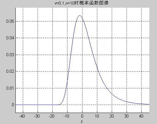 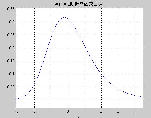 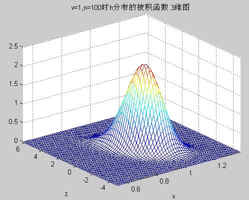 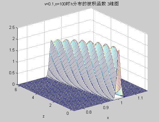 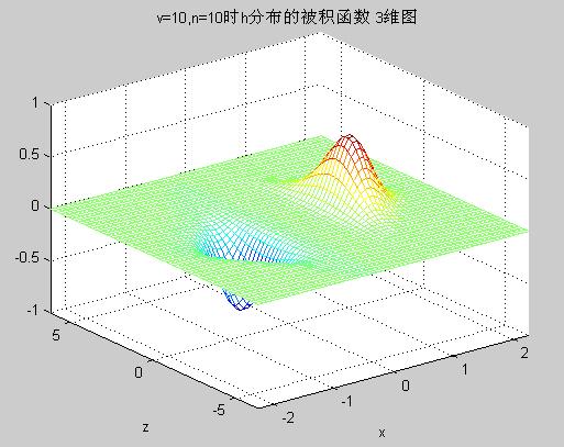 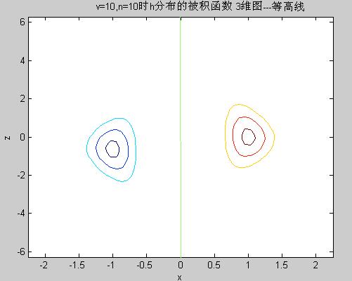 [ Last edited by plp626 on 2010-10-5 at 15:30 ] |
|
| Floor10 plp626 | Posted 2008-05-29 19:56 |
| 银牌会员 Posts 1,020 Credits 2,278 | |
|
```
% Print normal distribution table % $Author: plp626 Date: 2008-5-23 $ function f() % Main function, p=0:9; % p from 0 to 9 represents the second decimal place of the random variable value fprintf(' z ') for i=1:10 fprintf('%-8.1d',p(i)) end fprintf('\n') for z=0:0.1:2.0 % First decimal place fprintf('%4.1f',z) for i=1:1:10 fprintf('%8.4f',int_f(z+p(i)/100)) % Call int_f to calculate the probability value corresponding to z+p(i)/100. if i==10 fprintf('\n') end end end %%%%%%%%%%%%%%%%%%%%%%%%%%%%%%%%%%%%%%%%%%%%%%%%%%%% function r=int_f(a) % Function int_f calculates the probability (integral from negative infinity to a) syms x r=double(int(1/sqrt(2*pi)*exp(x^2/-2),-inf,a)); % int command calculates the integral, double command converts the calculation result to double type value and returns ``` |
|
| Floor11 plp626 | Posted 2008-05-30 22:39 |
| 银牌会员 Posts 1,020 Credits 2,278 | |
|
```
%%%%%%%%%%%%%%%%%%%%%%%%%%%%%%%%%%%%%%%%%%%%%%%%%%%%%%%%% %Probability function of coefficient of variation H {plp626|19:11 2008-5-24} %Given z, return the probability density. %r=pdfh(v,n,z) %v Coefficient of variation %n Degrees of freedom %z Random variable %%%%%%%%%%%%%%%%%%%%%%%%%%%%%%%%%%%%%%%%%%%%%%%%%%%%%%%%% function result=pdfh(v,n,z) if round(n)-abs(n)~=0||n==0 disp('error: Degrees of freedom can only take positive integers!') end xinf=2.5; %For cases where n>4, taking 2.5 is sufficient to ensure accuracy. If too large, quadl integration will fail. if n<4 xinf=4.5; end if round(n)-abs(n)==0&&n~=0 if v==0 disp('Current ν=0') result=gamma(n./2).*(1+(z.^2)./(n-1)).^(n./-2)./gamma((n-1)./2)./sqrt((n-1).*pi); result=double(result); else gm_n=((n-1)./2).^((n-1)./2)./sqrt(pi./2)./gamma((n-1)./2); syms x result=gm_n.*int(x.^(n-1).*exp(((n-1).*x.^2+(z.*x+sqrt(n).*(x-1)./v).^2)./-2),'x',0,xinf); result=double(result); end end ``` |
|
|
[ Contact the Union admin team -
中国DOS联盟 -
Standard version ] Sponsored by ifanr Inc | © 2001–2023 |