问题我已经解决了
我的论文题目:变异系数的参数估计(原创)
疯狂学习了半个月M软件,现在还不会用那个@什么匿名函数的命令,还有全局变量设定,
现在把毕业设计的程序贴出了大家共享下,程序那里不足,或错误望指出,我会感激不尽。
D:\MATLAB65\WORK\H分布
├─H分布上侧分位数表
│ date.txt
│ finda.m
│ findp.m
│ main.m
│ print_h.m
│ readme.txt
│
└─相关的函数图例
cdf_cont.m
cdf_mesh.m
plot_pdf.m
plot_pdfab.m
readme.txt
---------------------------------------------------------------------------------------------------------
---------- README.TXT
//** findp.m是独立程序,分别供finda.m与print_h.m调用 **//
findp.m 给定随机变量值求概率
参数列表(变异系数,自由度,随机变量值)
当n较大时(大于287)gm_n计算机直接显示inf(无穷大)所以287是计算机能计算的自由度上限
先对zint积分再对xquadl积分再另(ninf → ∞)这里ninf根据n,v取值,来确定∞。
由于函数的特殊性(在3附近已经极度减小,参考cdf3.m),
所以对ninf的取值可以大大减小计算时间,并保证精度。
finda.m 给定概率p反求分位数(随机变量值)
参数列表:(变异系数,自由度,概率值)
调用findp函数进行折半逼近,这里先变步长使得两个初值相对于概率P异号,然后折半逼近,
程序的效率很大程度上依赖于步长的增长系数K(不同的变异系数,自由度对这个系数比较敏感)以及findp函数的效率
得到一个4位精度的分位数平均需要20次的逼近。数据的可靠性取决于findp函数。
print_h.m 打印分布表
参数列表:(变异系数,自由度向量,概率向量)
程序依赖finda.m文件(计算指定概率的分位数),findp.m文件(计算随机变量a的概率值)
程序流程:调用finda函数求得指定概率的分位数然后制表打印
v 较大时与T分布表很接近,从数据上看H(+∞,n,a)=T(n+1,a)
比如v=1000时,H分布,自由度为20的分位数表就是T分布自由度为21的分位数表
程序用了inline函数,网上搜索知道这个函数会因为版本的问题第一次运行m文件报错,不管,clc后再运行一次,就不报错了。
---------- DATE.TXT
>> main
/** 变异系数为ν=0.10 的上侧分位数表 **/
─────────────────────────
n\p 0.5000 0.2500 0.0500 0.0050
─────────────────────────
2 6.8012 30.2295 211.3837 2242.6010
3 3.4702 14.9951 35.7568 35.7568
5 2.0402 9.9275 30.8079 76.2102
20 0.7967 6.4060 16.6854 26.4288
50 0.4824 5.7017 14.3829 24.3061
─────────────────────────
/** 变异系数为ν=1.00 的上侧分位数表 **/
─────────────────────────
n\p 0.5000 0.2500 0.0500 0.0050
─────────────────────────
2 0.5094 3.0323 21.6851 229.9287
3 0.2764 1.7483 6.9846 13.5901
5 0.1671 1.2971 4.0453 9.7534
20 0.0664 0.9746 2.5435 4.4741
50 0.0404 0.9091 2.2965 3.8206
─────────────────────────
/** 变异系数为ν=10.00 的上侧分位数表 **/
─────────────────────────
n\p 0.5000 0.2500 0.0500 0.0050
─────────────────────────
2 0.0361 1.1194 7.3685 75.4351
3 0.0223 0.8734 3.2109 11.1905
5 0.0142 0.7736 2.2639 4.9947
20 0.0059 0.7010 1.7741 2.9635
50 0.0036 0.6883 1.7046 2.7408
─────────────────────────
/** 变异系数为ν=1000.00 的上侧分位数表 **/
────────────────────────────────────────
n\p 0.5000 0.2500 0.1000 0.0500 0.0250 0.0100 0.0050
────────────────────────────────────────
2 0.0004 1.0011 3.0820 6.3237 12.7274 31.8756 63.7682
3 0.0002 0.8170 1.8872 2.9227 4.3072 6.9727 9.9370
4 -0.0002 0.7652 1.6388 2.3550 3.1850 4.5448 5.8466
5 0.0001 0.7410 1.5340 2.1331 2.7783 3.7498 4.6078
6 0.0001 0.7269 1.4765 2.0161 2.5720 3.3671 4.0350
7 0.0001 0.7178 1.4403 1.9440 2.4481 3.1445 3.7098
8 0.0001 0.7113 1.4154 1.8953 2.3657 2.9995 3.5015
9 0.0001 0.7066 1.3973 1.8602 2.3070 2.8979 3.3572
10 0.0001 0.7029 1.3834 1.8338 2.2631 2.8227 3.2515
11 0.0001 0.7000 1.3726 1.8131 2.2290 2.7650 3.1708
12 0.0001 0.6976 1.3638 1.7965 2.2018 2.7192 3.1072
13 0.0001 0.6956 1.3566 1.7828 2.1796 2.6820 3.0559
14 0.0001 0.6940 1.3505 1.7714 2.1611 2.6513 3.0135
15 0.0001 0.6926 1.3454 1.7618 2.1455 2.6254 2.9780
16 0.0001 0.6913 1.3409 1.7535 2.1321 2.6034 2.9478
17 0.0001 0.6903 1.3371 1.7464 2.1205 2.5844 2.9218
18 0.0001 0.6893 1.3336 1.7400 2.1104 2.5678 2.8992
19 0.0001 0.6885 1.3306 1.7345 2.1015 2.5532 2.8794
20 0.0001 0.6878 1.3280 1.7295 2.0936 2.5402 2.8619
21 0.0001 0.6871 1.3256 1.7251 2.0865 2.5287 2.8463
22 0.0001 0.6865 1.3234 1.7211 2.0802 2.5184 2.8322
23 0.0001 0.6859 1.3215 1.7175 2.0744 2.5091 2.8196
24 0.0001 0.6854 1.3197 1.7143 2.0692 2.5006 2.8082
25 0.0001 0.6850 1.3181 1.7113 2.0644 2.4928 2.7977
26 0.0001 0.6845 1.3165 1.7085 2.0600 2.4857 2.7882
27 0.0001 0.6842 1.3152 1.7060 2.0560 2.4793 2.7795
28 0.0001 0.6838 1.3139 1.7036 2.0523 2.4733 2.7714
29 0.0000 0.6834 1.3128 1.7014 2.0488 2.4677 2.7640
30 0.0000 0.6831 1.3117 1.6994 2.0457 2.4626 2.7571
31 0.0000 0.6828 1.3106 1.6976 2.0427 2.4578 2.7507
32 0.0000 0.6826 1.3096 1.6958 2.0399 2.4534 2.7448
33 0.0000 0.6823 1.3088 1.6942 2.0374 2.4492 2.7392
34 0.0000 0.6821 1.3079 1.6926 2.0349 2.4453 2.7340
35 0.0000 0.6818 1.3071 1.6912 2.0326 2.4417 2.7291
36 0.0000 0.6817 1.3064 1.6898 2.0305 2.4383 2.7244
37 0.0000 0.6815 1.3057 1.6886 2.0285 2.4350 2.7201
38 0.0000 0.6812 1.3050 1.6874 2.0266 2.4320 2.7160
39 0.0000 0.6811 1.3044 1.6862 2.0247 2.4291 2.7122
40 0.0000 0.6809 1.3038 1.6851 2.0230 2.4263 2.7085
41 0.0000 0.6807 1.3032 1.6841 2.0214 2.4237 2.7050
42 0.0000 0.6806 1.3027 1.6831 2.0199 2.4213 2.7018
43 0.0000 0.6804 1.3022 1.6822 2.0185 2.4190 2.6986
44 0.0000 0.6803 1.3017 1.6814 2.0170 2.4167 2.6957
45 0.0000 0.6802 1.3012 1.6805 2.0157 2.4146 2.6928
────────────────────────────────────────
---------- FINDA.M
%返回指定概率的分位数。
%参数列表:(变异系数,自由度,概率值)
%例finda(100,5,0.025)
function result=fun(v,n,p)
h=1; %初始步长
k=1; %步长增长系数k=1步长是线性增长,k>1时是几何级增长。
yihao=0; %异号标志
if v<1 || n<3 k=3; %v<1与n<3均值都完全偏离0附近。步长增长系数适当会大大减小折半逼近的次数!
end
a=0; %迭代初值
tmp=a; %tmp起记录a的作用
i=0;
%/*** 变步长迭代,异号时跳出循环 ***/
while findp(v,n,a)>p
tmp=a;
a=a+h;h=k*h;
yihao=1;
i=i+1;
end
while findp(v,n,a)<P
if yihao==1 break;
end
tmp=a;a=a-h;
h=k*h;
i=i+1;
end
b=tmp; %新的a值与tmp对应的概率相对P异号,将这个tmp传给b,下面进行折半逼近。
% /*** 折半逼近 ***/
while abs(a-b)>0.0001 %4位精度。
c=(a+b)/2;
i=i+1;
if (findp(v,n,c)-p)*(findp(v,n,a)-p)>0
a=c;
else
b=c;
end
end
%fprintf('循环次数:%d\n',i)
result=(a+b)/2;
---------- FINDP.M
%求h分布函数,随机变量的概率值
%参数列表(变异系数,自由度,随机变量值)
%例:
%findp(100,5,0)
function result=fun(v,n,a)
%/** xinf--设定积分区域
xinf=2.5; %对于n>4的情况取2.5即可保证精度。太大时quadl积分会失效。
if n<4 xinf=4.5;
end
if n > 280
disp('自由度太大会导致溢出错误')
end
if n>=2 && n<=280
syms x z ainf
gm_n=((n-1)/2)^((n-1)/2)/sqrt(pi/2)/gamma((n-1)/2);
f=x^(n-1)*exp((((n-1)*x^2+((z*x)+sqrt(n)*(x-1)/v)^2)/-2));
g=int(f,z,a,ainf); %先对z符号积分
h=subs(g,ainf,inf); %由于后面要用数值积分,这里不可以用h=limit(g,ainf,inf);
result=quadl(inline(h*gm_n),0,xinf); %积分区域为x=,z= 注意gm_n必须在inline(h*gm_n)里面,这样可以较少截断误差(否则逐级误差很大!)result=double(result);
end
if n<2
disp('自由度小于2时无意义')
end
%备注:
%自由度从22到23是个陡变。
---------- MAIN.M
p=;
n=;
print_h(0.1,n,p);
print_h(1,n,p);
print_h(10,n,p);
p=;
print_h(1000,2:45,p);
print_h(10000,2:45,p);
---------- PRINT_H.M
%打印h分布上侧分位数表
%参数列表:(变异系数,自由度向量,概率向量)
%自由度不能为1
%例:print_h(100,,)
function r=main(v,n,p)
fprintf('/** 变异系数为ν=%.2f 的上侧分位数表 **/\n',v)
xecho(length(p))
fprintf(' n\\p')
for i=1:length(p)
fprintf('%10.4f',p(i))
end
fprintf('\n')
xecho(length(p)) %调用xecho打印横线
for i=1:length(n)
fprintf(' %2.1d ',n(i))
for j=1:length(p)
fprintf('%10.4f',finda(v,n(i),p(j))) %调用finda函数(返回p(j)所对应的分位数)
if j==length(p) fprintf('\n')
end
end
end
xecho(length(p)) %调用xecho打印横线
%/*------------xecho--------------
function xecho(length)
for i=1:length*5+5
fprintf('─')
end
fprintf('\n')
%--------------------------------*/
-----------------------------------------------------------------------------
图例程序:
---------- README,TXT
每个文件都是独立程序。
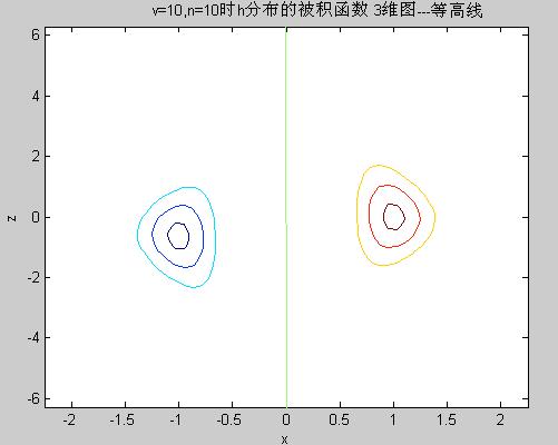
cdf_cont.m 输出分布函数的被积函数三维图像等高线
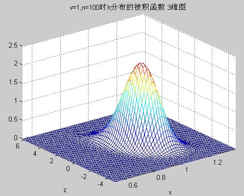
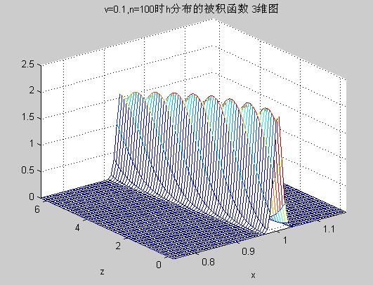
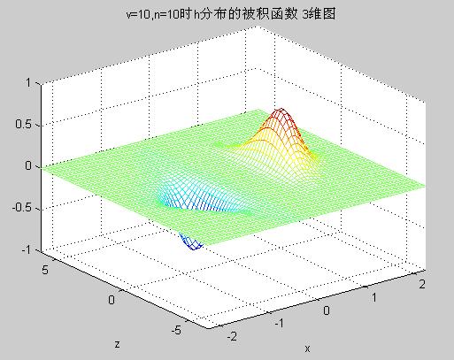
cdf_mesh.m 输出分布函数的被积函数三维图像网格线
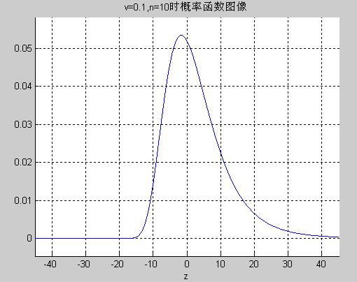
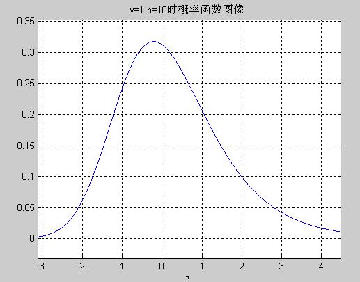
plot_pdf.m 输出概率密度函数图像
plot_pdfab.m 指定区间输出概率函数图像
plot_cdf.m 输出分布函数图像
帮助:
help
---------- CDF_CONT.M
%输出分布函数的被积函数3维图等高线
%参数列表:(变异系数向量,自由度向量)
%例:
%v=; %/*设置变异系数向量
%n=2:20,50:10:100;
%cdf_cont(v,n)
function main(v,n)
%v=0.026;n=2:20;
disp('按任意键继续...')
for i=1:length(v)
for j=1:length(n)
dgx(v(i),n(j))
pause %自动播放可用pause(0.4)
end
end
function r=dgx(v,n,a,b)
syms x z
gm_n=((n-1)/2)^((n-1)/2)/sqrt(pi/2)/gamma((n-1)/2);
f=x^(n-1)*exp((((n-1)*x^2+((z*x)+sqrt(n)*(x-1)/v)^2)/-2));
fxz=gm_n*f;
ezcontour(inline(fxz))
title()
---------- CDF_MESH.M
%输出不同h被积函数3维图。
%参数列表:(变异系数向量,自由度向量)
%例:
%v=;
%n=;
%cdf_mesh(v,n)
function main(v,n)
disp('按任意键继续...')
for i=1:length(v)
for j=1:length(n)
cdf3(v(i),n(j))
pause %自动播放可用pause(0.4)
end
end
%被积函数的二维图
%(变异系数,自由度)
function r=cdf3(v,n,a,b)
syms x z
gm_n=((n-1)/2)^((n-1)/2)/sqrt(pi/2)/gamma((n-1)/2);
f=x^(n-1)*exp((((n-1)*x^2+((z*x)+sqrt(n)*(x-1)/v)^2)/-2));
fxz=gm_n*f;
ezmesh(inline(fxz))
%meshc(inline(fxz),50)
title()
---------- PLOT_PDF.M
%打印h分布的概率函数图。
%参数列表:(变异系数向量,自由度向量)
%例:
%v=;
%n=;
%plot_pdf(v,n)
function main(v,n)
disp('正在拟合数据,稍等...')
hold on;grid on;
for i=1:length(v)
for j=1:length(n)
cdf2(v(i),n(j))
%pause %自动播放可用pause(0.4)
end
end
function result=cdf2(v,n)
xinf=2.5; %对于n>4的情况取2.5即可保证精度。太大时quadl积分会失效。
if n<4 xinf=4.5;
end
if n>=2 && n<=280
syms x z k
gm_n=((n-1)/2)^((n-1)/2)/sqrt(pi/2)/gamma((n-1)/2);
f=x^(n-1)*exp((((n-1)*x^2+((z*x)+sqrt(n)*(x-1)/v)^2)/-2));
h=inline(gm_n*int(f,'x',0,xinf));
ezplot(h)
title()
end
---------- PLOT_PDFAB.M
%指定区间,打印h分布的概率函数图。
%参数列表:(变异系数向量,自由度向量,)
%例:
%plot_pdfab(1,5,)
function main(v,n,x)
disp('正在拟合数据,稍等...')
for i=1:length(v)
hold off
for j=1:length(n)
hold on;grid on;
cdf2(v(i),n(j),x(1),x(2))
clc;disp('按任意键继续...')
pause %自动播放可用pause(0.4)
end
end
function result=cdf2(v,n,x1,x2)
xinf=2.5; %对于n>4的情况取2.5即可保证精度。太大时quadl积分会失效。
if n<4 xinf=4.5;
end
if n>=2 && n<=280
syms x z k
gm_n=((n-1)/2)^((n-1)/2)/sqrt(pi/2)/gamma((n-1)/2);
f=x^(n-1)*exp((((n-1)*x^2+((z*x)+sqrt(n)*(x-1)/v)^2)/-2));
h=inline(gm_n*int(f,'x',0,xinf));
ezplot(h,)
title()
end
Last edited by plp626 on 2010-10-5 at 15:30 ]
The problem has been solved.
My graduation thesis title: Parameter Estimation of the Coefficient of Variation (Original)
I studied software M crazily for half a month, but I still don't know how to use the command of @ anonymous function and the setting of global variables.
Now I post the graduation project program for everyone to share. If there are any deficiencies or errors in the program, please point them out. I will be very grateful.
D:\MATLAB65\WORK\H Distribution
├─Upper Quantile Table of H Distribution
│ date.txt
│ finda.m
│ findp.m
│ main.m
│ print_h.m
│ readme.txt
│
└─Related Function Figures
cdf_cont.m
cdf_mesh.m
plot_pdf.m
plot_pdfab.m
readme.txt
---------------------------------------------------------------------------------------------------------
---------- README.TXT
//** findp.m is an independent program, respectively called by finda.m and print_h.m **//
findp.m Find probability given random variable value
Parameter list (coefficient of variation, degrees of freedom, random variable value)
When n is large (greater than 287), gm_n is directly displayed as inf (infinity) by the computer, so 287 is the upper limit of degrees of freedom that the computer can calculate. First, integrate the z int, then integrate the x quadl, and then let (ninf → ∞). Here, ninf is determined according to the values of n and v. Due to the particularity of the function (it has extremely decreased near 3, refer to cdf3.m), the value of ninf can be greatly reduced to reduce the calculation time and ensure the accuracy.
finda.m Find quantile (random variable value) given probability p
Parameter list: (coefficient of variation, degrees of freedom, probability value)
Call the findp function for bisection approximation. Here, first change the step size to make two initial values have opposite signs relative to probability P, and then perform bisection approximation. The efficiency of the program largely depends on the step size growth coefficient K (different coefficients of variation and degrees of freedom are more sensitive to this coefficient) and the efficiency of the findp function.
On average, it takes about 20 approximations to get a 4-digit precision quantile. The reliability of the data depends on the findp function.
print_h.m Print distribution table
Parameter list: (coefficient of variation, degrees of freedom vector, probability vector)
The program depends on the finda.m file (calculate the quantile of the specified probability) and the findp.m file (calculate the probability value of random variable a)
Program flow: Call the finda function to obtain the quantile of the specified probability and then make a table and print it.
When v is large, it is very close to the T distribution table. From the data, H(+∞, n, a) = T(n+1, a)
For example, when v = 1000, the quantile table of the H distribution with degrees of freedom 20 is the quantile table of the T distribution with degrees of freedom 21.
The program uses the inline function. It is known from searching the Internet that this function may report an error when running the m file for the first time due to version issues. It doesn't matter. Run it again after clc, and it won't report an error.
---------- DATE.TXT
>> main
/** Upper quantile table with coefficient of variation ν = 0.10 **/
─────────────────────────
n\p 0.5000 0.2500 0.0500 0.0050
─────────────────────────
2 6.8012 30.2295 211.3837 2242.6010
3 3.4702 14.9951 35.7568 35.7568
5 2.0402 9.9275 30.8079 76.2102
20 0.7967 6.4060 16.6854 26.4288
50 0.4824 5.7017 14.3829 24.3061
─────────────────────────
/** Upper quantile table with coefficient of variation ν = 1.00 **/
─────────────────────────
n\p 0.5000 0.2500 0.0500 0.0050
─────────────────────────
2 0.5094 3.0323 21.6851 229.9287
3 0.2764 1.7483 6.9846 13.5901
5 0.1671 1.2971 4.0453 9.7534
20 0.0664 0.9746 2.5435 4.4741
50 0.0404 0.9091 2.2965 3.8206
─────────────────────────
/** Upper quantile table with coefficient of variation ν = 10.00 **/
─────────────────────────
n\p 0.5000 0.2500 0.0500 0.0050
─────────────────────────
2 0.0361 1.1194 7.3685 75.4351
3 0.0223 0.8734 3.2109 11.1905
5 0.0142 0.7736 2.2639 4.9947
20 0.0059 0.7010 1.7741 2.9635
50 0.0036 0.6883 1.7046 2.7408
─────────────────────────
/** Upper quantile table with coefficient of variation ν = 1000.00 **/
────────────────────────────────────────
n\p 0.5000 0.2500 0.1000 0.0500 0.0250 0.0100 0.0050
────────────────────────────────────────
2 0.0004 1.0011 3.0820 6.3237 12.7274 31.8756 63.7682
3 0.0002 0.8170 1.8872 2.9227 4.3072 6.9727 9.9370
4 -0.0002 0.7652 1.6388 2.3550 3.1850 4.5448 5.8466
5 0.0001 0.7410 1.5340 2.1331 2.7783 3.7498 4.6078
6 0.0001 0.7269 1.4765 2.0161 2.5720 3.3671 4.0350
7 0.0001 0.7178 1.4403 1.9440 2.4481 3.1445 3.7098
8 0.0001 0.7113 1.4154 1.8953 2.3657 2.9995 3.5015
9 0.0001 0.7066 1.3973 1.8602 2.3070 2.8979 3.3572
10 0.0001 0.7029 1.3834 1.8338 2.2631 2.8227 3.2515
11 0.0001 0.7000 1.3726 1.8131 2.2290 2.7650 3.1708
12 0.0001 0.6976 1.3638 1.7965 2.2018 2.7192 3.1072
13 0.0001 0.6956 1.3566 1.7828 2.1796 2.6820 3.0559
14 0.0001 0.6940 1.3505 1.7714 2.1611 2.6513 3.0135
15 0.0001 0.6926 1.3454 1.7618 2.1455 2.6254 2.9780
16 0.0001 0.6913 1.3409 1.7535 2.1321 2.6034 2.9478
17 0.0001 0.6903 1.3371 1.7464 2.1205 2.5844 2.9218
18 0.0001 0.6903 1.3336 1.7400 2.1104 2.5678 2.8992
19 0.0001 0.6885 1.3306 1.7345 2.1015 2.5532 2.8794
20 0.0001 0.6878 1.3280 1.7295 2.0936 2.5402 2.8619
21 0.0001 0.6871 1.3256 1.7251 2.0865 2.5287 2.8463
22 0.0001 0.6865 1.3234 1.7211 2.0802 2.5184 2.8322
23 0.0001 0.6859 1.3215 1.7175 2.0744 2.5091 2.8196
24 0.0001 0.6854 1.3197 1.7143 2.0692 2.5006 2.8082
25 0.0001 0.6850 1.3181 1.7113 2.0644 2.4928 2.7977
26 0.0001 0.6845 1.3165 1.7085 2.0600 2.4857 2.7882
27 0.0001 0.6842 1.3152 1.7060 2.0560 2.4793 2.7795
28 0.0001 0.6838 1.3139 1.7036 2.0523 2.4733 2.7714
29 0.0000 0.6834 1.3128 1.7014 2.0488 2.4677 2.7640
30 0.0000 0.6831 1.3117 1.6994 2.0457 2.4626 2.7571
31 0.0000 0.6828 1.3106 1.6976 2.0427 2.4578 2.7507
32 0.0000 0.6826 1.3096 1.6958 2.0399 2.4534 2.7448
33 0.0000 0.6823 1.3088 1.6942 2.0374 2.4492 2.7392
34 0.0000 0.6821 1.3079 1.6926 2.0349 2.4453 2.7340
35 0.0000 0.6818 1.3071 1.6912 2.0326 2.4417 2.7291
36 0.0000 0.6817 1.3064 1.6898 2.0305 2.4383 2.7244
37 0.0000 0.6815 1.3057 1.6886 2.0285 2.4350 2.7201
38 0.0000 0.6812 1.3050 1.6874 2.0266 2.4320 2.7160
39 0.0000 0.6811 1.3044 1.6862 2.0247 2.4291 2.7122
40 0.0000 0.6809 1.3038 1.6851 2.0230 2.4263 2.7085
41 0.0000 0.6807 1.3032 1.6841 2.0214 2.4237 2.7050
42 0.0000 0.6806 1.3027 1.6831 2.0199 2.4213 2.7018
43 0.0000 0.6804 1.3022 1.6822 2.0185 2.4190 2.6986
44 0.0000 0.6803 1.3017 1.6814 2.0170 2.4167 2.6957
45 0.0000 0.6802 1.3012 1.6805 2.0157 2.4146 2.6928
────────────────────────────────────────
---------- FINDA.M
% Return the quantile of the specified probability.
% Parameter list: (coefficient of variation, degrees of freedom, probability value)
% Example: finda(100,5,0.025)
function result=fun(v,n,p)
h=1; % Initial step size
k=1; % Step size growth coefficient k=1, step size is linearly increasing, and when k>1, it is geometrically increasing.
yihao=0; % Sign opposite flag
if v<1 || n<3 k=3; % When v<1 and n<3, the mean value completely deviates from near 0. The appropriate step size growth coefficient will greatly reduce the number of bisection approximations!
end
a=0; % Iteration initial value
tmp=a; % tmp is used to record a
i=0;
%/*** Variable step size iteration, jump out of the loop when signs are opposite ***/
while findp(v,n,a)>p
tmp=a;
a=a+h;h=k*h;
yihao=1;
i=i+1;
end
while findp(v,n,a)<P
if yihao==1 break;
end
tmp=a;a=a-h;
h=k*h;
i=i+1;
end
b=tmp; % The new a value has opposite sign relative to P compared with tmp, pass this tmp to b, and perform bisection approximation below.
% /*** Bisection approximation ***/
while abs(a-b)>0.0001 % 4-digit precision.
c=(a+b)/2;
i=i+1;
if (findp(v,n,c)-p)*(findp(v,n,a)-p)>0
a=c;
else
b=c;
end
end
%fprintf('Number of iterations:%d\n',i)
result=(a+b)/2;
---------- FINDP.M
% Find the probability value of the random variable of the h distribution function
% Parameter list (coefficient of variation, degrees of freedom, random variable value)
% Example:
% findp(100,5,0)
function result=fun(v,n,a)
%/** xinf--Set integration region
xinf=2.5; % For the case where n>4, take 2.5 to ensure accuracy. When too large, quadl integration will fail.
if n<4 xinf=4.5;
end
if n > 280
disp('Excessive degrees of freedom will lead to overflow error')
end
if n>=2 && n<=280
syms x z ainf
gm_n=((n-1)/2)^((n-1)/2)/sqrt(pi/2)/gamma((n-1)/2);
f=x^(n-1)*exp((((n-1)*x^2+((z*x)+sqrt(n)*(x-1)/v)^2)/-2));
g=int(f,z,a,ainf); % First perform symbolic integration on z
h=subs(g,ainf,inf); % Since numerical integration will be used later, here cannot use h=limit(g,ainf,inf);
result=quadl(inline(h*gm_n),0,xinf); % Integration region is x=, z= Note that gm_n must be inside inline(h*gm_n), so that the truncation error can be reduced (otherwise the error at each level is very large!) result=double(result);
end
if n<2
disp('It is meaningless when degrees of freedom are less than 2')
end
% Remarks:
% There is a sudden change from degrees of freedom 22 to 23.
---------- MAIN.M
p=;
n=;
print_h(0.1,n,p);
print_h(1,n,p);
print_h(10,n,p);
p=;
print_h(1000,2:45,p);
print_h(10000,2:45,p);
---------- PRINT_H.M
% Print the upper quantile table of the h distribution
% Parameter list: (coefficient of variation, degrees of freedom vector, probability vector)
% Degrees of freedom cannot be 1
% Example: print_h(100,,)
function r=main(v,n,p)
fprintf('/** Upper quantile table with coefficient of variation ν=%.2f **/\n',v)
xecho(length(p))
fprintf(' n\\p')
for i=1:length(p)
fprintf('%10.4f',p(i))
end
fprintf('\n')
xecho(length(p)) % Call xecho to print the horizontal line
for i=1:length(n)
fprintf(' %2.1d ',n(i))
for j=1:length(p)
fprintf('%10.4f',finda(v,n(i),p(j))) % Call the finda function (return the quantile corresponding to p(j))
if j==length(p) fprintf('\n')
end
end
end
xecho(length(p)) % Call xecho to print the horizontal line
%/*------------xecho--------------
function xecho(length)
for i=1:length*5+5
fprintf('─')
end
fprintf('\n')
%--------------------------------*/
-----------------------------------------------------------------------------
Figure program:
---------- README,TXT
Each file is an independent program.
cdf_cont.m Output contour of 3D image of the integrand of the distribution function
cdf_mesh.m Output mesh of 3D image of the integrand of the distribution function
plot_pdf.m Output image of the probability density function
plot_pdfab.m Output image of the probability function in the specified interval
plot_cdf.m Output image of the distribution function
Help:
help
---------- CDF_CONT.M
% Output contour of 3D image of the integrand of the distribution function
% Parameter list: (coefficient of variation vector, degrees of freedom vector)
% Example:
% v=; %/*Set coefficient of variation vector
% n=2:20,50:10:100;
% cdf_cont(v,n)
function main(v,n)
%v=0.026;n=2:20;
disp('Press any key to continue...')
for i=1:length(v)
for j=1:length(n)
dgx(v(i),n(j))
pause % Automatic playback can be used pause(0.4)
end
end
function r=dgx(v,n,a,b)
syms x z
gm_n=((n-1)/2)^((n-1)/2)/sqrt(pi/2)/gamma((n-1)/2);
f=x^(n-1)*exp((((n-1)*x^2+((z*x)+sqrt(n)*(x-1)/v)^2)/-2));
fxz=gm_n*f;
ezcontour(inline(fxz))
title()
---------- CDF_MESH.M
% Output 3D image of different h integrands.
% Parameter list: (coefficient of variation vector, degrees of freedom vector)
% Example:
% v=;
% n=;
% cdf_mesh(v,n)
function main(v,n)
disp('Press any key to continue...')
for i=1:length(v)
for j=1:length(n)
cdf3(v(i),n(j))
pause % Automatic playback can be used pause(0.4)
end
end
% 2D image of the integrand
%(coefficient of variation, degrees of freedom)
function r=cdf3(v,n,a,b)
syms x z
gm_n=((n-1)/2)^((n-1)/2)/sqrt(pi/2)/gamma((n-1)/2);
f=x^(n-1)*exp((((n-1)*x^2+((z*x)+sqrt(n)*(x-1)/v)^2)/-2));
fxz=gm_n*f;
ezmesh(inline(fxz))
%meshc(inline(fxz),50)
title()
---------- PLOT_PDF.M
% Print the image of the probability function of the h distribution.
% Parameter list: (coefficient of variation vector, degrees of freedom vector)
% Example:
% v=;
% n=;
% plot_pdf(v,n)
function main(v,n)
disp('Fitting data, please wait...')
hold on;grid on;
for i=1:length(v)
for j=1:length(n)
cdf2(v(i),n(j))
%pause % Automatic playback can be used pause(0.4)
end
end
function result=cdf2(v,n)
xinf=2.5; % For the case where n>4, take 2.5 to ensure accuracy. When too large, quadl integration will fail.
if n<4 xinf=4.5;
end
if n>=2 && n<=280
syms x z k
gm_n=((n-1)/2)^((n-1)/2)/sqrt(pi/2)/gamma((n-1)/2);
f=x^(n-1)*exp((((n-1)*x^2+((z*x)+sqrt(n)*(x-1)/v)^2)/-2));
h=inline(gm_n*int(f,'x',0,xinf));
ezplot(h)
title()
end
---------- PLOT_PDFAB.M
% Print the image of the probability function of the h distribution in the specified interval.
% Parameter list: (coefficient of variation vector, degrees of freedom vector, )
% Example:
% plot_pdfab(1,5,)
function main(v,n,x)
disp('Fitting data, please wait...')
for i=1:length(v)
hold off
for j=1:length(n)
hold on;grid on;
cdf2(v(i),n(j),x(1),x(2))
clc;disp('Press any key to continue...')
pause % Automatic playback can be used pause(0.4)
end
end
function result=cdf2(v,n,x1,x2)
xinf=2.5; % For the case where n>4, take 2.5 to ensure accuracy. When too large, quadl integration will fail.
if n<4 xinf=4.5;
end
if n>=2 && n<=280
syms x z k
gm_n=((n-1)/2)^((n-1)/2)/sqrt(pi/2)/gamma((n-1)/2);
f=x^(n-1)*exp((((n-1)*x^2+((z*x)+sqrt(n)*(x-1)/v)^2)/-2));
h=inline(gm_n*int(f,'x',0,xinf));
ezplot(h,)
title()
end
Last edited by plp626 on 2010-10-5 at 15:30 ]